Clustering teams by their defense p2

November 14, 2016

This is the second part of my cluster analysis of NBA teams. In this paper I am looking for groups of teams based on their opponents percentages from certain areas on the court. I use slightly different methods than in previous analysis, not only just to try it out, but I found out that every method result in divergent clusters and in this case following algorithm suit me the best.

Data

I created five standarized variables based on original efficiency columns. Bear in mind, that those percentages do not include garbage time, which I consider as unnecessary noise. We can call it like “significant game time percentage” or something similar. Final dataset looks like this:

	team	lr.ef	mr.ef	pa.ef	ra.ef	tr.ef	lr.efnorm	mr.efnorm	pa.efnorm	ra.efnorm	tr.efnorm	abr
1	Atlanta Hawks	37.93	38.04	39.92	56.70	33.77	-1.2311723	-1.7127106	0.3156051	-1.4372570	-1.201666	ATL
2	Boston Celtics	39.76	38.79	36.81	60.01	33.70	-0.0735878	-1.2074531	-1.0946418	-0.0568564	-1.253632	BOS
3	Brooklyn Nets	41.35	41.02	41.09	63.03	37.03	0.9321823	0.2948458	0.8461481	1.2026028	1.218493	BKN

Reducing dimensionality

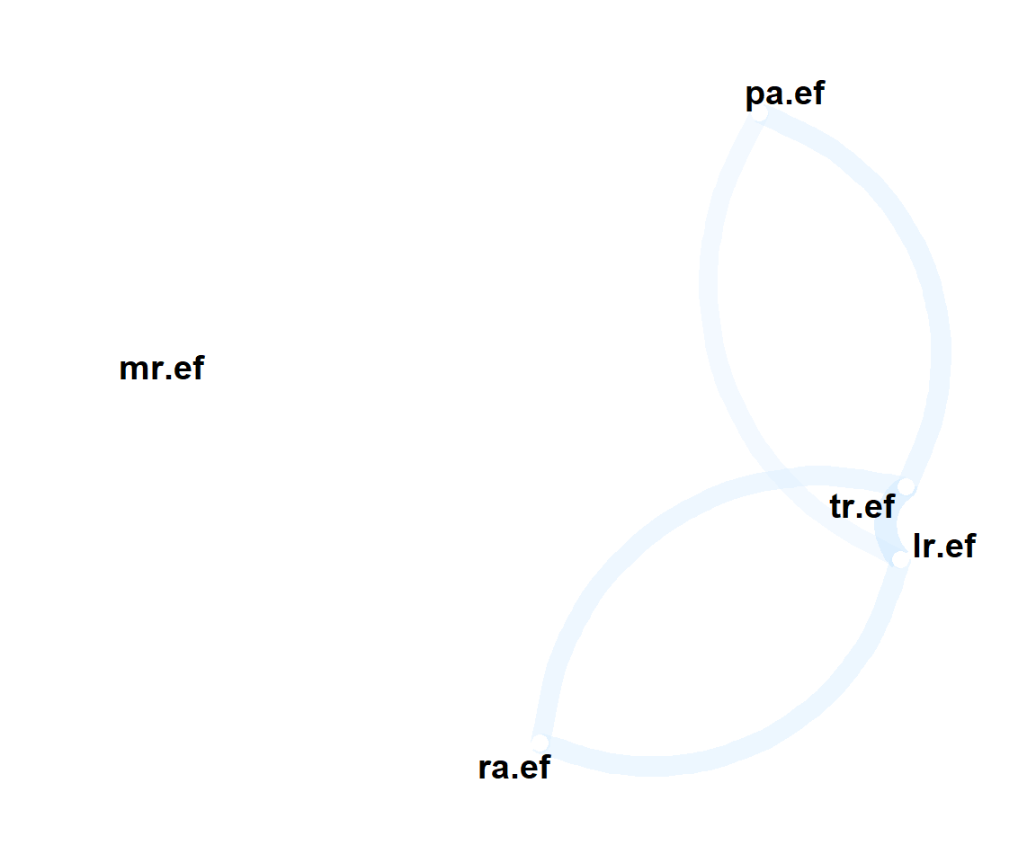
There is high probability that for most defenders there is no difference if they are guarding in mid-range or in long-range zone. Let’s check if there are significant collinearities between some variables.

I used package corr for nice visualization:

## # A tibble: 5 x 6
##   rowname   lr.ef    mr.ef   pa.ef  ra.ef   tr.ef
##   <chr>     <dbl>    <dbl>   <dbl>  <dbl>   <dbl>
## 1 lr.ef   NA        0.0155   0.305  0.378  0.479 
## 2 mr.ef    0.0155  NA      - 0.138  0.276  0.0223
## 3 pa.ef    0.305  - 0.138   NA      0.106  0.370 
## 4 ra.ef    0.378    0.276    0.106 NA      0.358 
## 5 tr.ef    0.479    0.0223   0.370  0.358 NA

Thick redish lines indicate negative correlations between variables. Collinearities at the level above 45% indicate that model would benefit from reducing number of dimensions.

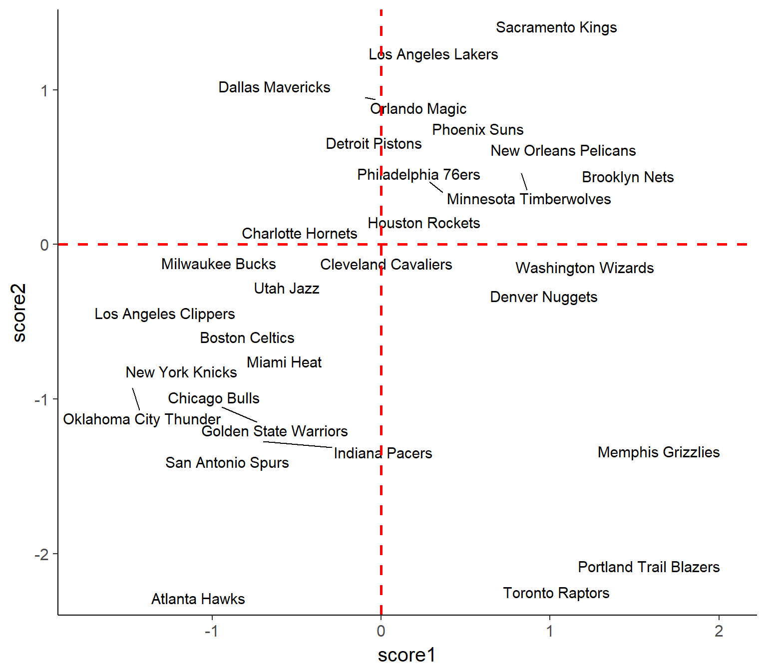
Over-dimensionality can be reduced by applying Factor Analysis algorithm, among others, and it is exactly what I am going to do. Chart below presents how newly formed factors (score1, score2) explain the variance across teams.

Hierarchical clustering

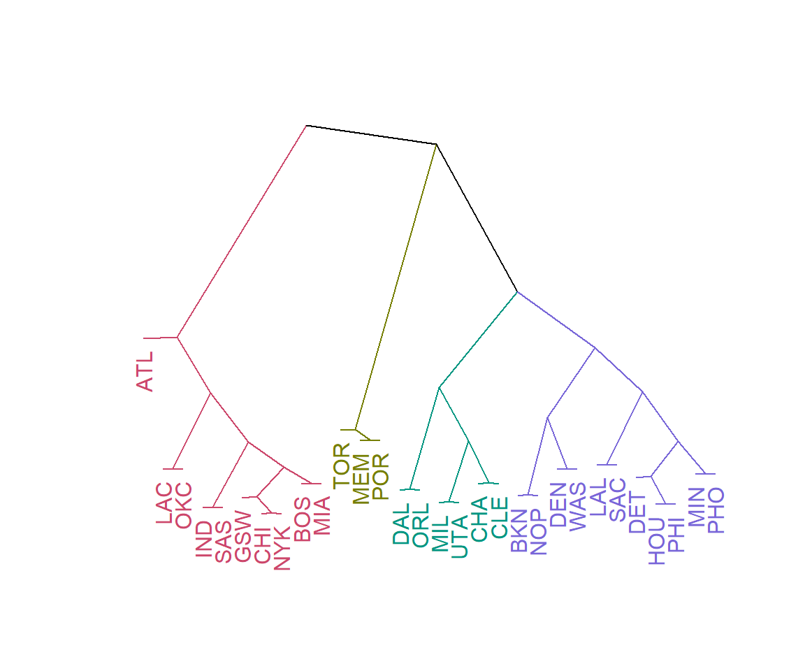
Across all methods I found the “complete” hierarchical clustering working the best for my data. It helped me to avoid combining teams that defend poorly in the same zone, but one of them defends poorly everywhere, and the other one is totally ok in the rest of the areas. I called it a Rocket-Cavaliers case. Brilliant.

Insights

Lets take a moment and appreaciate Atlanta Hawks, because this team is in class of its own in terms of defense efficiency. They are next to the group of really good defensive teams which include Spurs, almost-champs, athletic OKC, a couple of smart teams with great coaches and - barely - lazy in regular season NBA champions Cleveland Cavaliers.

The group of Raptors, Grizzlies and Blazers consists of 3 outliers, which is easily confirmed by DBSCAN algorithm.

There is 13-team cluster containing many teams which finished outside of playoffs or left them early (Dallas, Houston, Detroit) or they lie just at the deepest of bottoms (Phoenix, Philly, Brooklyn, Sacramento… its going on.)