NBA Machine Learning #3 - Splines, LOESS and GAMs with mlr package
About series
So I came up with an idea to write series of articles describing how to apply machine learning algorithms on some examples of NBA data. Got to say that plan is quite ambitious - I want to start with machine learning basics, go through some common data problems, required preprocessing tasks and obviously, algorithms. Starting with Linear Regression and hopefully finishing one day with Neural Networks or any other mysterious blackbox. Articles are going to cover both theory and practice (code) and data will be centered around NBA.
Most of the tasks will be done with mlr package since I try to master it and I am looking for motivation. Datasets and scripts will be uploaded on my github, so feel free to use them for own practice!
- 1. Process of building a model
- 2. Linear Regression with mlr package
- 3. Splines, LOESS and GAMs with mlr package
library(tidyverse)
library(broom)
library(mlr)
library(GGally)
library(visdat)

options(scipen = 999)

nba <- read_csv("../../data/mlmodels/nba_linear_regression.csv") %>% glimpse
## Observations: 78,739
## Variables: 13
## $ PTS <int> 23, 30, 22, 41, 20, 8, 33, 33, 28, 9, 15, 24, 21, ...
## $ FG2A <int> 10, 17, 12, 14, 8, 7, 24, 12, 13, 11, 12, 13, 13, ...
## $ FG3A <int> 3, 3, 3, 6, 1, 2, 1, 4, 0, 2, 1, 0, 0, 2, 1, 3, 1,...
## $ FTA <int> 4, 9, 2, 21, 14, 4, 10, 15, 7, 4, 6, 5, 6, 12, 13,...
## $ AST <int> 5, 6, 1, 6, 10, 6, 3, 3, 6, 8, 4, 8, 4, 5, 7, 5, 7...
## $ OREB <int> 0, 2, 2, 1, 2, 0, 2, 4, 1, 0, 2, 0, 2, 1, 6, 0, 0,...
## $ PF <int> 5, 4, 1, 3, 5, 2, 2, 4, 3, 3, 3, 4, 2, 1, 2, 3, 5,...
## $ TOV <int> 5, 4, 4, 5, 2, 1, 0, 6, 4, 3, 6, 1, 1, 0, 1, 6, 2,...
## $ STL <int> 2, 0, 2, 2, 1, 1, 4, 4, 1, 0, 0, 2, 0, 2, 4, 5, 0,...
## $ PACE <dbl> 104.44, 110.01, 94.88, 103.19, 92.42, 93.35, 106.2...
## $ MINS <dbl> 35.0, 33.9, 36.1, 41.6, 34.4, 36.7, 39.9, 34.5, 35...
## $ PLAYER_NAME <chr> "Giannis Antetokounmpo", "Giannis Antetokounmpo", ...
## $ GAME_DATE <date> 2017-02-03, 2017-02-04, 2017-02-08, 2017-02-10, 2...PTS <- nba %>% pull(PTS)
FG2A <- nba %>% pull(FG2A)
FTA <- nba %>% pull(FTA)Introduction
Based on the result of previous model I decided to give up on using classic linear regression and try my luck in fitting other methods to the data I got. Analyzes of previous model indicated strong skewness and higher variance for observations with larger response values (it was heteroscedaskicity) and I am going to try to address that issue with the family of additive regression functions - Splines, Local Regression and Generalized Additive Models. The approach for all of them is quite similar, hence they are covered in one article. Let’s start!
Splines
Spline is a function defined piecewise by polynomials… it’s first sentence of method describtion and I am already overwhelmed. Piecewise means that the function has different formula for each interval. That means f(x) can be equal to 3 for x lower than 3 and then f(x) might be equal to 2x for x greater or equal to 0.
Polynomial is expression consisting of substracted/added/exponentially modified variables, for example f(x) x^2 + 3x.
Let’s try to tackle another part… We are using splines to interpolate real function. Splines are calculated between each 2,3,4,…, n points. Dependent on which splines we choose, we need different number of data points (linear function has 2 parameters, so we need 2 points, quadratic has 3 and uses 3, cubic requires 4).
Remember that splines need x variables to be sorted in ascending order before they are computed.
Linear spline
That is just linear function connecting 2 points:
\[ linear spline (x) = y(x_1) + \frac{y(x_2) - y(x_1)}{x_2 - x_1} (x-x_1) \] where X belongs to <X1, X2>
Having points (x1,y1) and (x2,y2) we can calculate function above and receive linear spline for range between those two points.
It’s very simple straight line interpolation, but disadvantage of it is that we don’t use information from any other observations except those two. Also slope of interpolation is discontinued (data point is likely to have different slope on each side). To avoid those problems we want to use some more complex interpolation.
Quadratic spline
Quadratic spline interpolates curve between 2 points, that is computed in the way to provide continuity of slope on data points. Each spline is quadratic equations with 3 unknows:
\[ y(x) = ax^2 + bx + c \] Hence there are 3 coefficients to be computed we need to have 3 equations to do so. First 2 equations come obviously from borderline data points (x1,y1),(x2,y2) and the third one is provided by continuity condition. Quadratic splines model requires slopes to be equal on interior points, when interior point is finish point for first spline and start point for the second spline.
So when we have 100 observations, we need to calculate 99 splines, each one of them contains 3 coefficients hence we need 297 equations overall to do so.
- 198 equations are the result of using data points (external ones are used only once)
- 98 equations are the result of matching derivatives from the left and right handside of a data point
- One last coefficient we get by assuming that the first or the last spline is linear, so we presume a is equal to 0. We have to do this, otherwise problem will be mathematically impossible to solve.
Spline 0:
\[ y_0 = b_0x_0 + c_0\] \[ y_1 = b_1x_1 + c_1\]
Continuity of slope, calculated for internal point (x1,y1)
\[ 2a_0x_1 + b_0 = 2a_1x_1 + b_1\]
Spline 1:
\[ y_1 = a_1x_1^2 + b_1x_1 + c_1\] \[ y_1 = a_1x_2^2 + b_1x_2 + c_1\]
Continuity of slope, calculated for internal point (x2,y2)
\[ 2a_1x_2 + b_1 = 2a_2x_2 + b_2\]
And it goes on…
Cubic spline
Most often used method. Uses cubic funtion to create spline interpolating real function behind the data. Thanks to comparing second derivatives, we make sure the general function is smoothed even better on internal points.
\[ y(x) = ax^3 + bx^2 + cx + d \]
We use equations in similar fashion to the quadratic splines, but here we need to compare second derivatives as well.
So when we have 100 observations, we need to calculate 99 splines, each one of them contains 4 coefficients hence we need 496 equations overall to do so.
- 198 equations are the result of using data points (external ones are used only once)
- 98 equations are the result of matching first derivatives from the left and right handside of a data point
- 98 equations are the result of matching second derivatives from the left and right handside of a data point
- 2 equations for endpoints, assuming that second derivatives of starting and finishing observation are equal to 0.
First derivative:
\[ y'(x) = 3ax^2 + 2bx + c \]
Second derivative:
\[ y''(x) = 6ax + 2b\]
Natural condition for endpoints:
\[ S''(a)=S''(b)=0. \]
Example
Let’s now run an example with spline regression using bs() function. Bs here stands for b-spline, just to be clear. It’s advantage is that can be ran with lm function (but not mlr package at this moment, since it is not supporting formula objects)
For bs() there are 3 important hyperparameters: - knots: specified points when function will be changed - degree: degree of polynomial - default is 3 to get cubic splines - df: degrees of freedom: if specified, chooses knots at suitable quantiles (can be used instead of knots)
How to find optimal hyperparameter? You either know whats the best set of knots can be, or just use cross validation.
lm_bs <- lm(PTS ~ splines::bs(FG2A, df = 6), data = nba)
broom::tidy(lm_bs)
## term estimate std.error statistic
## 1 (Intercept) 1.435588 0.06169867 23.26773
## 2 splines::bs(FG2A, df = 6)1 1.365031 0.12383747 11.02276
## 3 splines::bs(FG2A, df = 6)2 4.148201 0.11043365 37.56283
## 4 splines::bs(FG2A, df = 6)3 7.862334 0.09270323 84.81187
## 5 splines::bs(FG2A, df = 6)4 23.770708 0.23796098 99.89330
## 6 splines::bs(FG2A, df = 6)5 30.732711 0.65448885 46.95681
## 7 splines::bs(FG2A, df = 6)6 48.384056 1.43346075 33.75332
## p.value
## 1 0.000000000000000000000000000000000000000000000000000000000000000000000000000000000000000000000000000000000000000000000023847324683513225281224212626085545707610435783863067626953125000000000000000000000000000000000000000000000000000000000000000000000000000000000000000000000000000000000000000000000000000000000000
## 2 0.000000000000000000000000000311287484096202606898874665208865053500630892813205718994140625000000000000000000000000000000000000000000000000000000000000000000000000000000000000000000000000000000000000000000000000000000000000000000000000000000000000000000000000000000000000000000000000000000000000000000000000000000
## 3 0.000000000000000000000000000000000000000000000000000000000000000000000000000000000000000000000000000000000000000000000000000000000000000000000000000000000000000000000000000000000000000000000000000000000000000000000000000000000000000000000000000000000000000000000000000000000000000000000000000000000000000004531909
## 4 0.000000000000000000000000000000000000000000000000000000000000000000000000000000000000000000000000000000000000000000000000000000000000000000000000000000000000000000000000000000000000000000000000000000000000000000000000000000000000000000000000000000000000000000000000000000000000000000000000000000000000000000000000
## 5 0.000000000000000000000000000000000000000000000000000000000000000000000000000000000000000000000000000000000000000000000000000000000000000000000000000000000000000000000000000000000000000000000000000000000000000000000000000000000000000000000000000000000000000000000000000000000000000000000000000000000000000000000000
## 6 0.000000000000000000000000000000000000000000000000000000000000000000000000000000000000000000000000000000000000000000000000000000000000000000000000000000000000000000000000000000000000000000000000000000000000000000000000000000000000000000000000000000000000000000000000000000000000000000000000000000000000000000000000
## 7 0.000000000000000000000000000000000000000000000000000000000000000000000000000000000000000000000000000000000000000000000000000000000000000000000000000000000000000000000000000000000000000000000000000000000000000000000000000000000000000000000000000000057057733175785530829043912248721426294650882482528686523437500000Local Regression (LOESS)
Local regression is non-parametric method trying to make a prediction for a data point using observations that are in near that point. This concept is very similar to well-known k-nearest neighbours.
Local Regression algorithm iteratively goes through all observations and for each one (i.e. focal point per iteration) picks k nearest points to fit line or curve using OLS algorithm in that window. We are choosing the size of this window using cross validation.
Another thing to remember is the fact that points are weighted using kernel function, so the closest points are more important than the points that are further from the focal point.
After first, initial full prediction on whole training dataset, local regression goes through all points once again, this time to weight observations by the initial error terms i.e. the larger error term value, the lower weight because it is indicator of an outlier, that should not be taken into consideration for fitting data.
data(economics, package="ggplot2")  # load data
economics$index <- 1:nrow(economics)  # create index variable
economics <- economics[1:80, ]  # retail 80rows for better graphical understanding
loessMod10 <- loess(uempmed ~ index, data=economics, span=0.10) # 10% smoothing span
loessMod25 <- loess(uempmed ~ index, data=economics, span=0.25) # 25% smoothing span
loessMod50 <- loess(uempmed ~ index, data=economics, span=0.50) # 50% smoothing span


smoothed10 <- predict(loessMod10)
smoothed25 <- predict(loessMod25)
smoothed50 <- predict(loessMod50)

plot(economics$uempmed, x=economics$date, type="l", main="Loess Smoothing and Prediction", xlab="Date", ylab="Unemployment (Median)")
lines(smoothed10, x=economics$date, col="red")
lines(smoothed25, x=economics$date, col="green")
lines(smoothed50, x=economics$date, col="blue")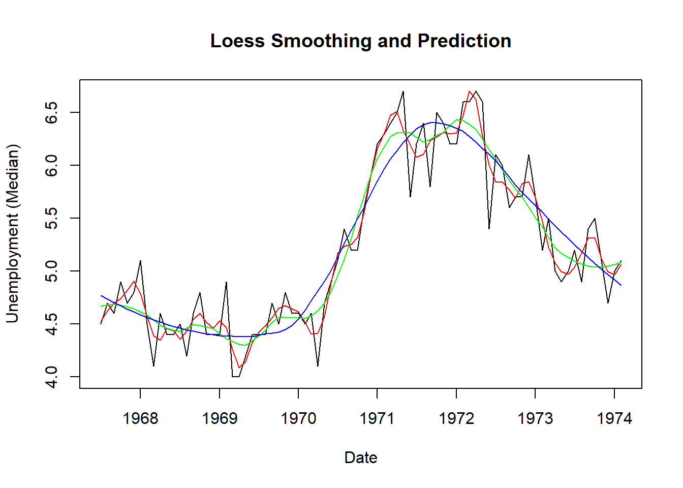
Generalized Additive Models (GAMs)
Generalized additive models are extension of general linearized models, which are extension of general linear model (I think I will cover differences in the next article - please find me NBA related variable that has pure poisson distribution).
GAMs are very flexible method that applies parametric, nonparametric or spline transformation to each predictor before fitting the model (in which response can be transformed as well). It’s a way to fit data of many various distributions together and receive fine model. One big disadvantage is that they can be easily overfit - various nonparametric methods like splines can fit to the noise pretty fast, so we all have to be very cautious.
I wish that one day I will write a paragraph which would have first letters of rows combining into ‘cross validation’.
\[g(y) = β0 + f1(x1) + f2(x2) +…+ fn(xn)\]
Once we got to know splines concept, GAMs are really simple to understand, but let’s see how this model is actually fitted, because (as in splines example) it might not be that obvious.
Training GAMs
– to do:
- example for loess
- gams example and training (ols?)
- proper NBA tryout