NBA Machine Learning #1 - Introduction to modelling

Visual analysis

univariate analysis

• Plotting distributions of numerical variables (density and histogram plots)
• Barplots to check frequencies of categories

 nba %>% ggplot() + geom_density(aes(x = FG2A))  + theme_bw() +
    theme(
          axis.text.x=element_text(hjust=1,size = 12, face = 'bold'),
          axis.text.y=element_text(size = 12, face = 'bold'),
          axis.title.y = element_blank()
          ,panel.grid = element_blank())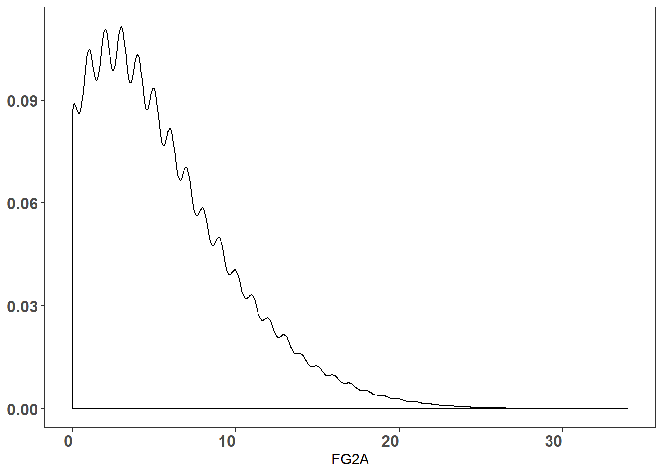

multivariate analysis

• Scatterplots and correlation plots to find dependencies between numerical variables
• Boxplots of categorical variables and dependent variable in order to find useful dummy variables

 nba %>%
  slice(1:1000) %>%
ggpairs(columns = 2:4) + theme_bw()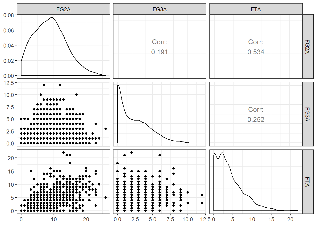

Data cleaning

Do you have a lot of categorical variables? Do you have dates? Sneaky numerical ID columns? Outlying values caused by error? Useless text variables ? Missing values????

Those 1 or 2 annoying observations with missing values that you haven’t spotted…

Most of issues above can be easily spotted during visual analysis, but it’s good to have one more look at the whole dataset:

visdat::vis_dat(nba[1:1000,])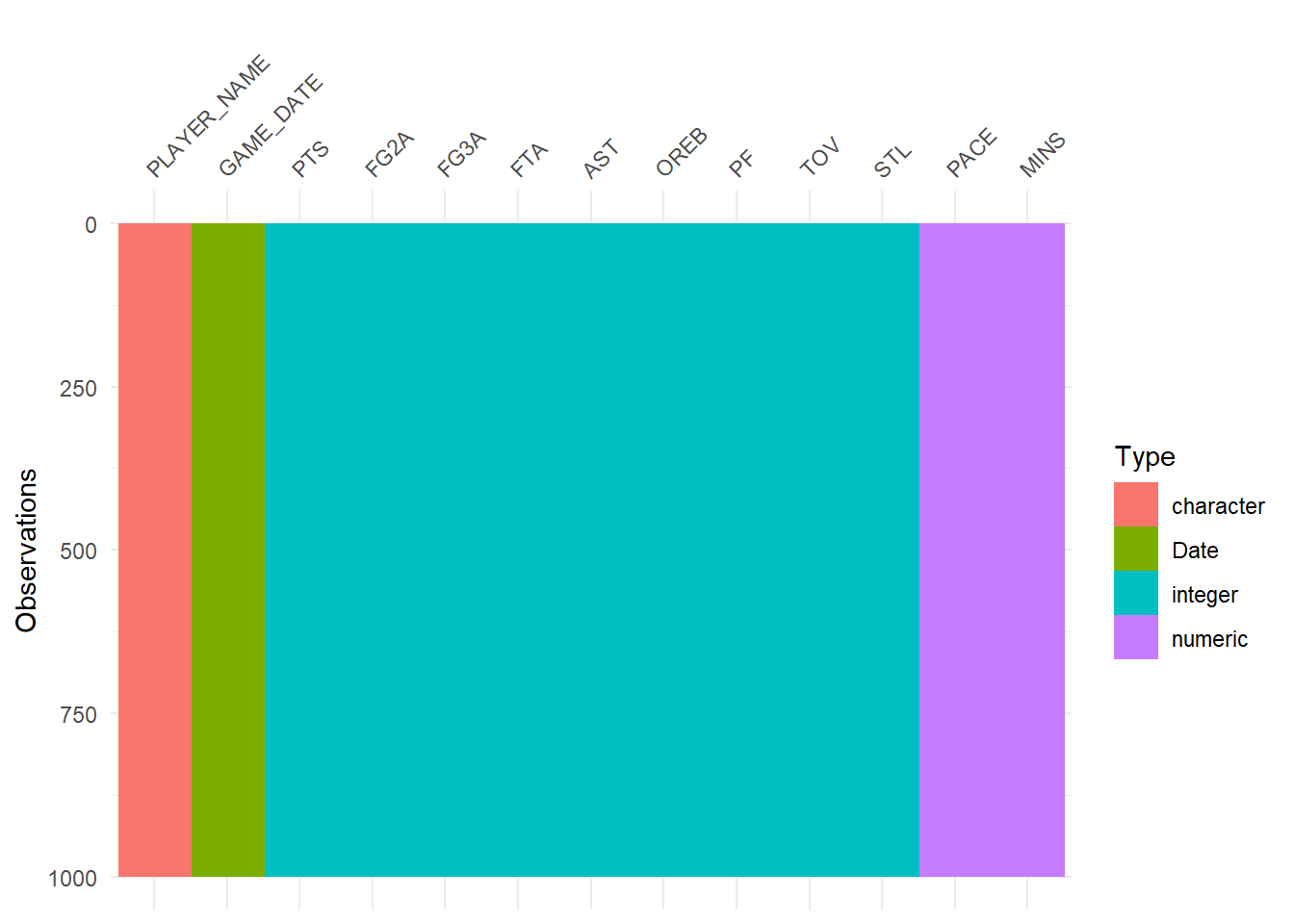

Just to name a few data cleaning tasks (you probably won’t need all of them everytime). There will be article only about those tasks and when to use them.

• normalisation
• standarisation
• scalling
• log-scalling
• binning
• dealing with outliers
• imputing empty values

Feature engineering

Again, this is bread and butter of data science. In the end how you prepare your data is way more important for the overall model score than algorithm that you chose. Winners of every Kaggle competition repeat it regularly that obtaining the right variables was the crucial factor that gave them the advantage.

Proper feature engineering is close to art. You need to use your domai expertise, instincts, data analysis and tries to find what will work. There is no one proper way here.

• how to transform continuous variables
• what’s the best split for categorical variables to create dummy ones
• shall I use dimensionality reduction techniques
• shall I combine some variables

Feature selection

Once again, you can pick variables yourself, but there is high chsnce you will be better off with some standard approaches like using statistical analysis or feature selection algorithms:

• correlation analysis
• permutation tests
• family of entropy and information gain tests
• elastic net approach for regression models
• gridsearch
• stepwise search

Just to name a few. All of them have their pros and cons, and it’s definately good to know them. It’s important to mention that there are methods that are capable of dealing with unimportant variables themselves, but I still wouldn’t recommend leaving them in dataset. This would add unnecessary noise to the data and also slow down the learning process, which is not perfect. Always aim for the best!

Class imbalance

This can be huge if you miss that problem before applying algorithm. If there is large difference (lets say 0.70 to 0.30) between class frequencies in dependent variable, it can lead to false model predictions. As always there are several ways of dealing with it, dependent mostly on number of observations of your training dataset and accordingly number of observations per class.

• If number of observations is huge/sufficient then you can cut the number of observations from major class
• If opposite.. well, then you have to use algorithms to generate new data in order to equalize frequencies. Methods will be covered in further article.

After we got to know our data, managed to process it and select variables we want to use, it’s finally time for some time!

Why one should always start with simpler solutions?

Although I know how tempting it is to just grab tons of variables, perform feature selection, throw them into model bowl and get effortless result, it might be better to start your modelling with some simple approach and then build gradually on top of that.

There are several reasons to do that:

• You understand your data better. By picking variables manually (based on domain knowledge/common sense) you easily get to know which features play most important role in defining independent variable.

• Model is easier to explain. It’s especially important if you just became data scientist for a company ( :) ) and you need to make other people believe in your theories and analysis. It shows that you know what you are doing. Simple proof of concepts enable non-technical stakeholders to understand the idea behind, understand that it is going in right direction and then they will be eager to wait for more complex solutions.

This argument is more important than you think and way more important than you would like it to be.

• There is a chance that if you pick best features and process them right way, you will receive high quality model with some minimal amount of work. Let’s say we build very simple predictor of Points, using 2 points field goal attempts and three point field goal attempts. (Respectively FG2A and FG3A)

very_simple <- lm(PTS ~ FG2A  + FG3A, nba)

broom::glance(very_simple)[c('r.squared','adj.r.squared')]

##   r.squared adj.r.squared
## 1 0.7711777     0.7711719

Model returns R squared of 0.77, which is decent in respect of how much time we spend on building the model (obviously its on training dataset without any validation but still, you get an idea…). It won’t win you a competition on Kaggle, but it will give you solid foundation for further work.

data.frame(real_values = nba$PTS, predictions = very_simple$fitted.values, Game_Player = paste(nba$PLAYER_NAME, nba$GAME_DATE)) %>%
  slice(52400:52550) %>%
  tidyr::gather(key = 'Variable', value = 'Value', - Game_Player) %>%
  ggplot() +
    geom_line(aes(x = Game_Player, y = Value, group = Variable, color = Variable), size = 1) + theme_bw() +
    theme(
          axis.text.x=element_text(angle=45,hjust=1,size = 3, face = 'bold'),
          axis.text.y=element_text(size = 12, face = 'bold'),
          axis.title = element_blank()
          ,legend.position='top'
          ,panel.grid = element_blank())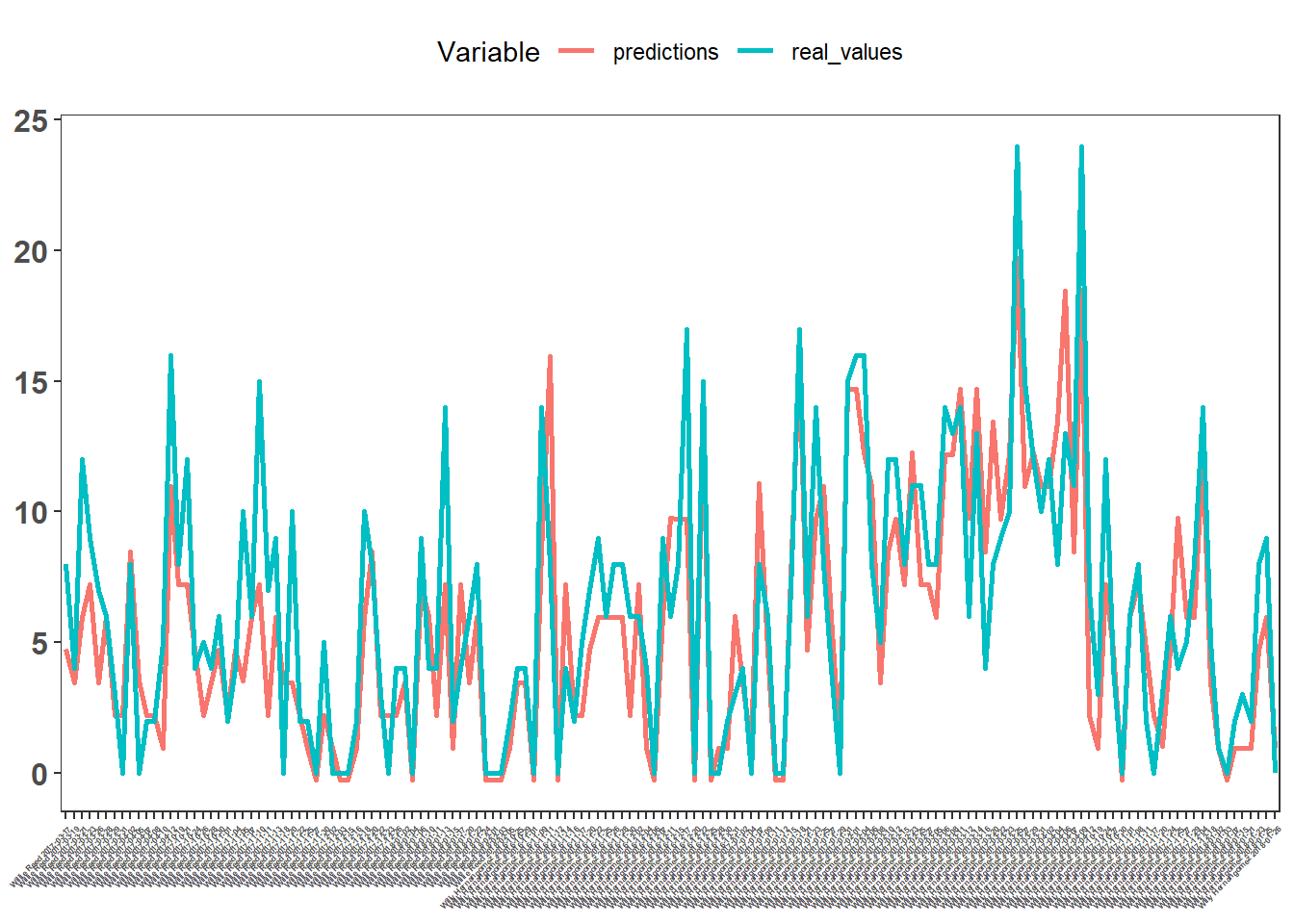

It’s far from perfect, but we got something we can build on.

It has its cons as well:

• Yes, it takes time. Especially with large number of variables to consider and when you think about all possible feature engineering methods you can try out. But in the end this is data science job - searching for a real signal somewhere in the data.

• It’s totally possible that simple model is not able to cover problem in any way - situation just requires more complex ones (for example necessary variable combinations). Then the simple approach will never give us anything promising. Then well… at least we gain that information.

Bias - Variance tradeoff

Remember that, even though you can build decent model with very simple solution, you should not stop in that point. There is high risk of model being biased. Bias is caused by model making wrong or too simple assumptions about real dependencies occuring in real world.

Imagine if we try to apply linear model on a problem that is highly non-linear. Algorithm will try to fit coefficients to data as best as it can, but even though errors will be minimized, predictions on validation datasets won’t be accurate due to wrong assumptions about reality. That happens because model uses wrong function to describe reality.

What you can do to reduce bias error, is to add more information to the model. Feed it with more observations and more variables so the function will get more complex and will fit better to the data. New learnt function will be definately better reflection of real world.

Unfortunately the more complex the function the higher the variance error becomes. It means that model became so good at fitting training dataset, it is not general enough to predict values for new, never seen before observations. This is called overfitting.

Variance indicates how much the model will change if it trained on new dataset.

During model building you need to remeber about that problem. Your model will perform the best when you find the optimal point between Bias and Variance. Model cannot be too simple because the vias will be very high, in the same time it can’t be overcomplicated, because it will cause high variance and overfitting.

High bias is a problem for parametric algorithms like linear and logistic regression, on the other hand nonparametric models like KNN or Decision Trees have low bias because they don’t assume parametric dependencies. However, those models tend to have high variance. Your goal during building supervised learning model is to achieve low bias and low variance.

Bootstrapping

Bias can be reduced by adding more variables to a model or using nonparametric method. Then we can try to reduce variance by using one of many bootstrap approaches.

• Most common one is using random forest instead of decision trees
• You can also run bagging/ensemble versions of other algorithms
• There are also several versions of Cross-validation that can be used here
• One can stack many different models and then take an average of them to provide final prediction

There are a lot of possibilities…