NBA Machine Learning #2 - Linear Regression with mlr package

Ordinary Least Squares - OLS

One predictor

The basic and most common estimation method for linear regression. It’s based on minimizing the sum of distances between actual response observations and set of predictors. In other words, minimazing residual sum of squares RSS.

RSS - residual sum of squares

\[ RSS = \sum{(y_i - \hat{y_i})^2} \]

If we use formula for model prediction:

\[ \hat{y} = b_0 + b_nx_n \]

\[ RSS = \sum_{i = 1}^{n}{(y_i - (b_0 + b_nx_n)_i)^2} \]

Our goal is to minimize RSS, knowing y and x values - that means that we have to find b0 and bn parameters that will minimize RSS. We do that by using derivatives (RSS is a function of b0 and bn, minimum is when the slope of function is equal to 0, derivative finds slope at given point).

We are reaching the scary point here!

• Partial derivative of RSS by b0 (intercept):

\[ -2\sum_{i=1}^{n}{(y_i - (b_0 + b_1x_i) )} \]

• Partial derivative of RSS by b1 (x1 coefficient)

\[ -2\sum_{i=1}^{n}{(y_i - (b_0 + b_1x_1i) )x_1i} \]

• We need to find minimum of a function - this is the place when derivative is equal to 0

\[ -2\sum_{i=1}^{n}{(y_i - (b_0 + b_1x_i) )} = 0 \]

\[ -2\sum_{i=1}^{n}{(y_i - (b_0 + b_1x_i) )x_i} = 0 \]

• Which gives us pair of equations to calculate our coefficients b0 and b1. After some steps of math calculations we should get:

\[ b_1 = - \frac{n\bar{x}\bar{y} - \sum{yx}}{\sum{x^2 - n\bar{x^2}}}\]

…or just…

\[ b_1 = \frac{COV(x,y)}{VAR(x)} \]

…and…

\[ b_0 = \bar{y} - b_1\bar{x}\]

…As a last piece of simple linear regression formula.

Where n is number of observations, x is predictor variable, y is response variable.

So, in easier to read, coding example:

• response: PTS
• predictor: FG2A

n = length(PTS)

b1 <- - (mean(PTS)*mean(FG2A)*n - sum(PTS*FG2A))/(sum(FG2A^2) - n*mean(FG2A)^2)
b0 <- mean(PTS) - b1*mean(FG2A)

cat(paste('b0 = ',round(b0,4),'b1 =',round(b1,4)))

## b0 =  2.1704 b1 = 1.3956

or

cov(FG2A,PTS)/var(FG2A)

## [1] 1.395591

We get slope and coefficient of simple linear regression. Let’s compare it with built-in R function:

lm(PTS ~ FG2A)

## 
## Call:
## lm(formula = PTS ~ FG2A)
## 
## Coefficients:
## (Intercept)         FG2A  
##       2.170        1.396

Coefficients match and that is very good news!

More predictors (matrix-based formula)

Now it’s time to present the solution for multiple linear regression. When we have more than one predictor it is MUCH easier to use matrix-based formula.

\[ \beta = (X^tX)^{-1}X^tY \] Where Beta stands for coefficients, X for matrix of predictors, Y for vector of response variable. Key thing! Add 1 as intercept to the X matrix if you try to calculate OLS manually, otherwise coefficients will not match the LM() function, which is quite annoying.

(Yes. It took me some time to realize it)

x <- nba %>%
  select(FG2A, FTA) %>%
  mutate(intercept = 1) %>%  
  as.matrix()

y <- nba %>% pull(PTS)

solve(t(x)%*%x)%*%t(x)%*%y

##                [,1]
## FG2A      1.0868669
## FTA       0.9940133
## intercept 1.7486047

Also, we have to remember that R uses QR decomposition for matrices, to make the numerical calculation more stable. So the most often used formula is:

\[ \beta = R^{-1}Q^tY\]

qrm <- qr(x)
solve(qr.R(qrm))%*%t(qr.Q(qrm))%*%y

##                [,1]
## FG2A      1.0868669
## FTA       0.9940133
## intercept 1.7486047

Let’s check with R function again!

lm(PTS ~ FG2A + FTA)

## 
## Call:
## lm(formula = PTS ~ FG2A + FTA)
## 
## Coefficients:
## (Intercept)         FG2A          FTA  
##       1.749        1.087        0.994

Coefficients seem to match again, which makes me really happy.

Stochastic Gradient Descent method

This is second estimation method I would like to present. Still not as common as OLS for linear regression models. But it’s very important to know it, especially because it is used in many others algorithms (neural networks for example). It’s advantegous when we have very large amount of data or when it is very sparse. Stochastic Gradient descent is also quite effective when we have multicollinearity in out data.

Gradient descent is algorithm minimizing functions. Given starting set of parameters, algorithm iteratively moves towards the best set of parameters (resulting in function minimum). On each step algorithm calculates gradient on one observation, and then updates coefficients. There are variations of that approach, mostly using batches of observations and/or iterations of process above.

Given simple linear regression, we are looking to minimize error of algorithm by optimizing slope and intercept parameters.

\[ MSE = \frac{1}{n}\sum_{i = 1}^{n}{(y_i - (b_0 + b_nx_n)_i)^2} \] Where MSE is mean squared error, b0 is intercept, bn is a slope.

Once again, we are looking for function gradients and we will find them using partial derivatives:

\[ \theta = \frac{-2}{n}\sum_{i=1}^{n}{(y_i - (b_0 + b_nx_i) )}\]

\[ \theta = \frac{-2}{n}\sum_{i=1}^{n}{(y_i - (b_0 + b_nx_i) )x_i}\] Every iteration will update the coefficients by the gradient value multiplied by learning rate. It will be repeated till algorithm converges. Each step consists of one data point or set of them, dependent on the specific version of algorithm. Learning rate is there to control the pace of modifications. We don’t want to make too big changes at each step, because we can miss the local minimum.

\[ \theta_{new} = \theta_{start} - L_{earning}R_{ate} * \theta_{gradient} \]

Code below shows implementation of Stochastic Gradient Descent. Starting points are intercept and slope both equal to -1. Learning rate is set to 0.04, why not. Gradient is calculated in a loop (soRRy) for each one of i observations. Animation will show prediction for every 5000 step.

library(gganimate)
library(ggplot2)

n = length(PTS)
intercept = -1
slope = -1
LR = 0.04

prediction <- intercept + slope*FG2A
ds_show <- data.frame(prediction, FG2A, PTS, intercept, slope, step = 0, stringsAsFactors = F)

i <- 1
for(i in 1:n){
  
  slope <- slope - LR*(-2/n)*sum(PTS[i]*FG2A[i] - intercept*FG2A[i] - slope*FG2A[i]^2)
  intercept <- intercept - LR*(-2/n)*sum(PTS[i] - intercept - slope*FG2A[i])
  

  if(i %% 5000 == 0){
      prediction <- intercept + slope*FG2A
      ds_stage <-  data.frame(prediction, FG2A, PTS, intercept, slope, step = i, stringsAsFactors = F)
      ds_show <- bind_rows(ds_show,ds_stage)
  }

  
}

animated <- ggplot(data = ds_show, aes(frame = step)) +
  geom_line(aes(x = FG2A,y = prediction), color = 'red')  + 
  geom_point(aes(x = FG2A,y = PTS), color = 'blue')  + 
  theme_bw()

gganimate(animated)

Stochastic Gradient Descent presentation

Linear relationship

We assume that there is linear and additive relationship between explonatory data and outcome variable. If we apply linear model to non-linear problem in real world, we get high-biased model.

ggplot()+
  geom_point(aes(x = PTS, y = FG2A)) + theme_bw()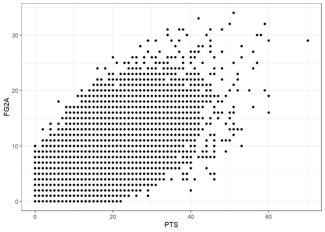

Scatter rlot above presents linear relationship between 2 variables. It indicates that we can use linear regression to predict one from another. It’s also good to calculate correlation.

 cor(FG2A, PTS)

## [1] 0.7718064

Correlation

Correlation is statistical measure of how strong is linear relationship between 2 variables. It doesn’t imply causation, as every statistics person likes to say. It’s quite useful metric for finding right variables for linear regression, when we want to have predictors highly correlated with repsonse variable, but not correlated with each other (to avoid multicollinearity).

Pearson’s correlation formula:

\[ cor(x,y) = \frac{cov(x,y)}{sd(x)sd(y)} \]

where cov is covariance and sd stands for standard deviation.

Pearson’s correlation can take value from range <-1;1> where 0 stands for no correlation, -1 for perfect negative correlation and 1 for perfect positive correlation.

Homoscedasticity of error terms

This always makes me ask a question:

Was it really necessary?

Was coming up with word that has 17 letters that much more efficient than calling it Constant variance?

Why can’t we just call it constant variance and enjoy simpler life when we use words that we understand, not trying to look snobbish?

Anyway, it’s called homoscedasticity and it means constant variance across observations. If variance changes with observations, then we get heteroscedasticity and it’s not good for our model. We can see it on residuals plot:

ds <- nba %>%
  select(PTS,FG2A, FG3A, FTA) %>%
  arrange(FG2A) %>%
  as.data.frame()

slr <- lm(PTS ~ FG2A, ds)
plot(slr, which = 3)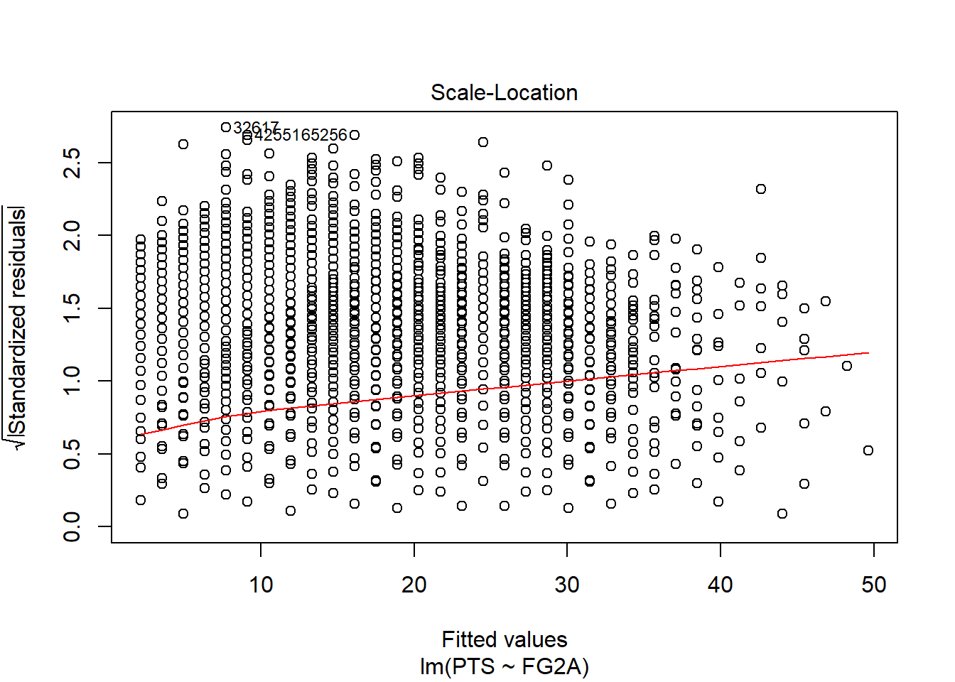

Plot above shows that unfortunately our simple regression model has heteroscedkadt…. it doesn’t have constant variance with increasing X. Error terms are getting bigger with increasing predictor. That means that our model is ok when it predicts on lower values, but is getting worse when independent variable increases.

I can tell you that it means that our estimator is no longer blue, or OLS assumption is wrong…but the most important information for us is now that fact that our model is not fitted perfectly:

• Model is worse than goodness of fit measures indicate
• Predictions on larger values have larger errors, so we can no longer be highly confident in predictions
• We need to use transformed variable (log-scaled, scaled, etc.) instead of basic one.

Important to note, that everytime we witness something different from complete randomness in residuals, then we know that our predictors are missing something.

Statistical tests for homoscedaskicity:

Breush-Pagan test

Idea behind this test is to run regression model which residuals of base model are standing for response on independent predictors.

null hypothesis: homoscedaskicity alternative: heteroscedaskicity

lmtest::bptest(slr)

## 
##  studentized Breusch-Pagan test
## 
## data:  slr
## BP = 2952.1, df = 1, p-value < 0.00000000000000022

P-value is super small, so we reject null hypothesis, which confirms non-constant variance

Dealing with heteroscedaskicity in the model:

We need to either transform variables or use weighted OLS to estimate model’s coefficients.

Weighted OLS

It means weighing observations to reduce impact of larger values, for example doing:

slr_w = lm(PTS ~ FG2A, data = ds, weights = 1/(FG2A))

Log Scaling predictor

slr_log = lm(PTS ~ log(FG2A), data = ds)

Normal distribution of error terms

We can check if residauls are normally distributed by looking at residuals vs fitted values plot. Ideally scatter points would have common shape across all fitted variables, meaning that the numbers are random. Below you can see that it is not a case. There is significant trend in how residuals values are decreasing when fitted values increase.

plot(slr$fitted.values,slr$residuals)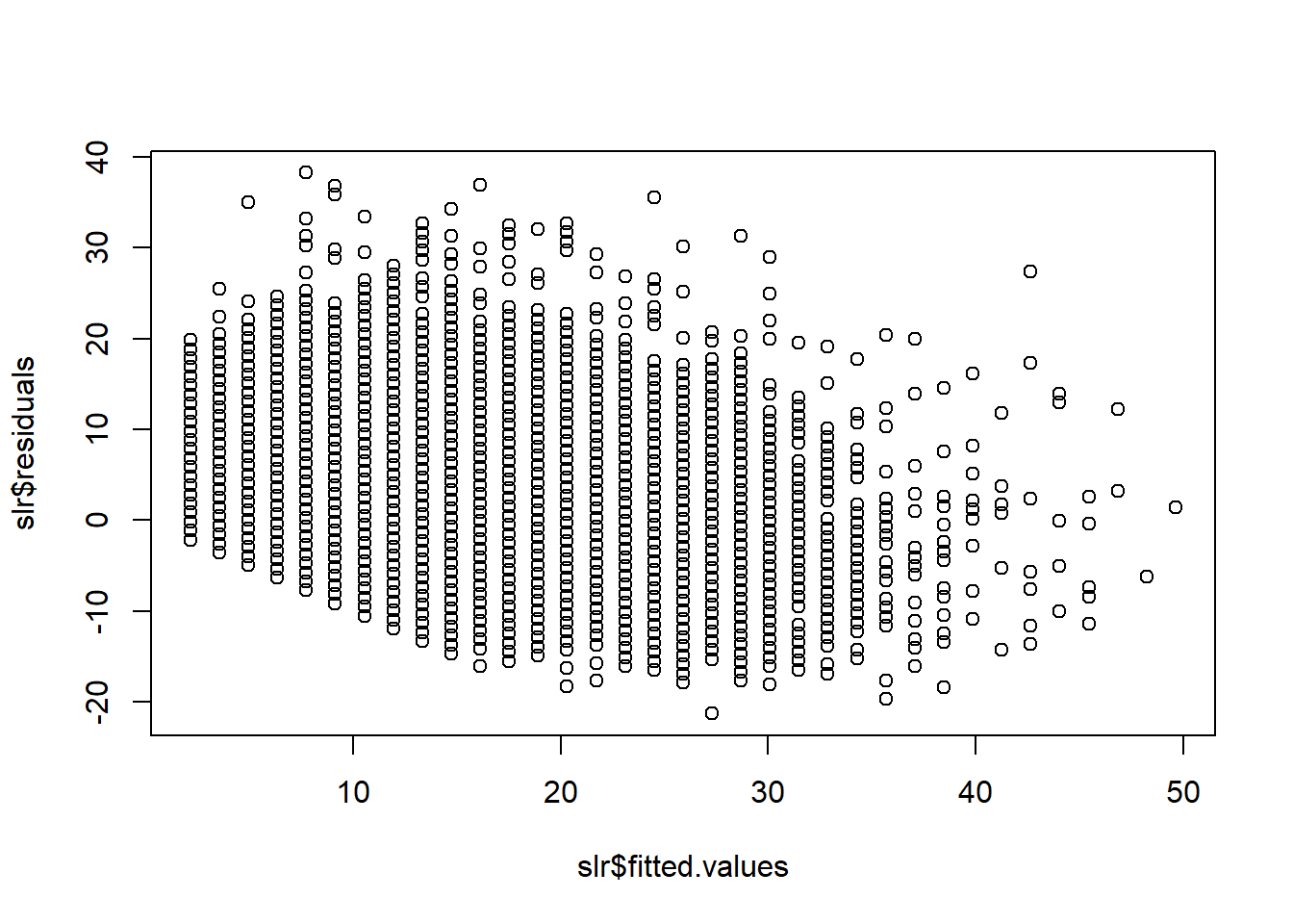

We can also use quantile-quantile (real vs theoretical quantiles) plot of residuals:

plot(slr, which = 2)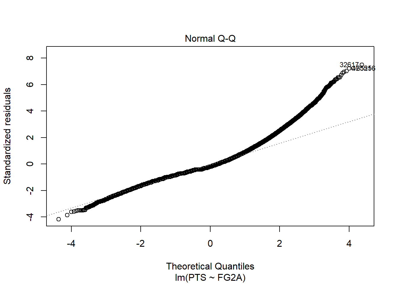

Which shows even better that residuals are not normally distributed and that is big problem for our model.

Statistical tests for normal distribution:

Shapiro-Wilk test

This test is biased by sample size i.e. the larger the sample the higher chance to get statistically significant result (always look on q-q plot)

null hypothesis: residuals normally distributed alternative: residuals are not normally distributed

shapiro.test(slr$residuals[1:5000])

## 
##  Shapiro-Wilk normality test
## 
## data:  slr$residuals[1:5000]
## W = 0.5889, p-value < 0.00000000000000022

In example above we reject the null hypothesis and confirm non-normality that visualizations presented above.

There are more statistical tests for normality added in nortest package, its worth checking and using more than one test for comparisons.

Autocorrelation of error terms

Autocorellation happens when residuals are dependent on previous residuals values (there is regression between current residual and its lagged values).

If a model is affected by autocorellation, than we know that are predictors are missing some important signal that was included in residuals. We probably need to add some new predictor.

Residual plot with autocorellation presents obvious trend going on.

Statistical tests for autocorrelation:

Durbin-Watson test

DW statistic checks what part of all residuals is covered by lagged values.

Durbin-Watson statistic lies in range between 0 and 4 with critical values Dl AND Du

• 0:Dl -> positive autocorrelation
• Dl:Du -> no autocorrelation
• Du:4 -> negative autocorrelation

lmtest::dwtest(slr)

## 
##  Durbin-Watson test
## 
## data:  slr
## DW = 1.4629, p-value < 0.00000000000000022
## alternative hypothesis: true autocorrelation is greater than 0

So to all of this simple linear regression model’s problems I need to add autocorrelation as well.

While building linear regression we need to always remember about residual graphs. Non-normal distribution, heteroscedaskicity and autocorrelation are things we need to account for and avoid while building the model. They make predictions less confident, error terms are growing or are falsely low, we might lacking some important information in the data.Always check residual graphs.

No Multicollinearity

If predictors are correlated with each other then it’s hard to tell which one really is significant in predicting response values. It can also add negative noise to coefficients during model training, so it is always good to check for correlation between independent variables.

First what we can do is to use correlation matrix before model training, and then pick variables that are highly correlated with response and not correlated with any other predictors.

cm <- cor(nba[,1:8])
corrplot::corrplot(cm, method = 'number', diag = F, type = 'upper') #plot matrix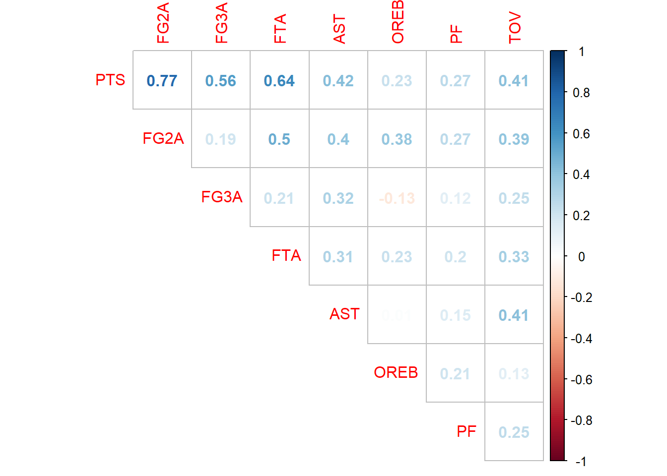

Obviously when we have lots of variables the only thing we can do is program the selection or use

Variance Inflation Factors

VIF is the ratio of variance in a model with multiple predictors, divided by the variance of a model with only one predictor. It presents magnitude of multicollinearity of each variable.

It is assumed that if value is larger than 5 then there is a problem and that variable should be removed or combined with correlated one.

ds_vif <- nba %>%
  select(PTS,FG2A, FG3A, FTA, AST, OREB, PF, TOV) %>% as.data.frame()

slr_vif <-  lm(PTS ~ ., data = ds_vif)

car::vif(slr_vif)

##     FG2A     FG3A      FTA      AST     OREB       PF      TOV 
## 1.746619 1.195806 1.407422 1.408611 1.284540 1.134261 1.372683

Since all of those predictors are close to one, they can stay in the model for now. If VIF gets closer to 5, then we can start worrying about multicollinearity.

Outliers

slr_show_any_outlier_plz <- lm(PTS ~ FTA, data = nba)
plot(slr_show_any_outlier_plz$residuals)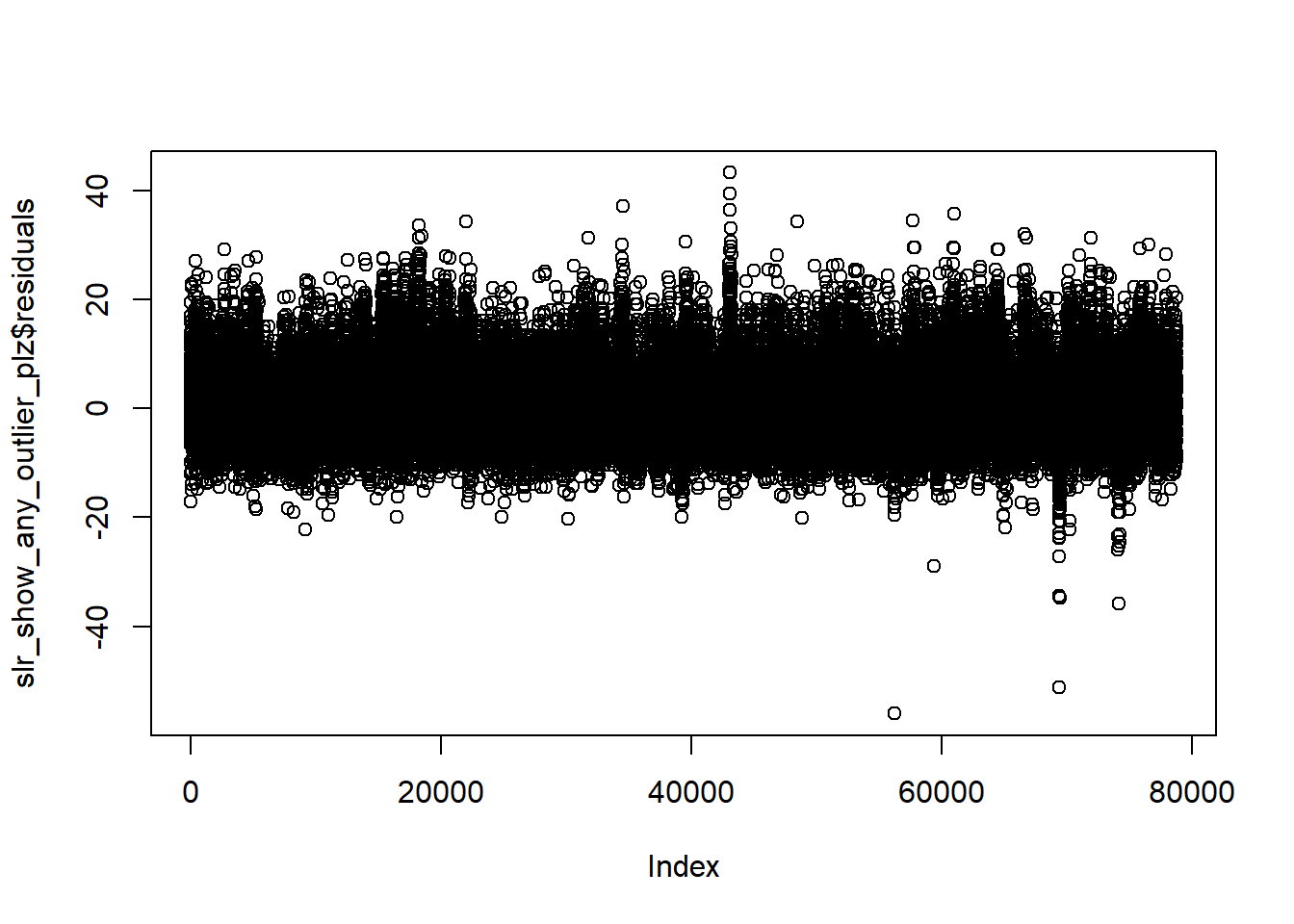

Built one poor model for purpose to show you that residuals plot can also be used to find outliers in the data.

Outliers are observations which response variable values are far away from the mean (there are different methods for tagging outliers - 3 standard deviations, interquantile range, median absolute deviations etc.). Some machine learning techniques are quite outlier-proof, but linear regression is not one of them. If you keep outlying observations in dataset, model still will try to fit them into general regression line creating skewed line.

It’s good to inspect why we got so extreme values in a dataset. Of course sometimes it is proper observation, but other times it can be caused by human or system error and therefore it should be cut from dataset or updated. Common technique is to impute mean/median value instead of outlier.

If we feel we have enough observations it might be easier to just remove it.

Initially to find outliers we can use density plots and/or boxplots to highlight them.

boxplot(nba$PTS)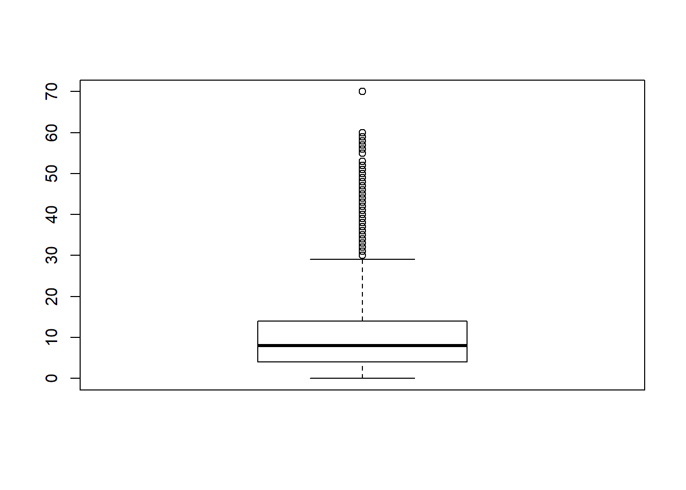

plot(density(nba$PTS))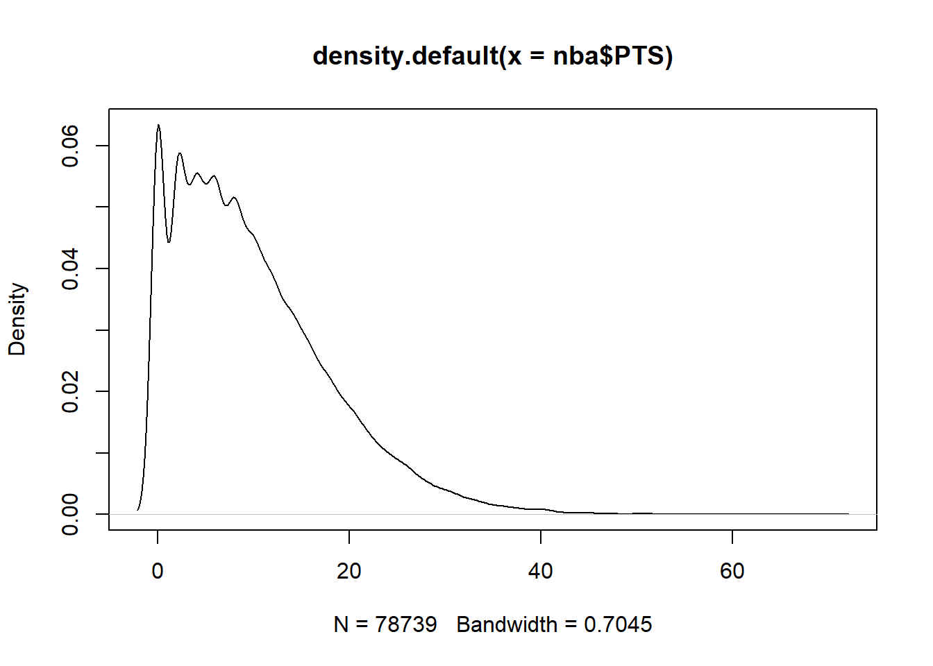

Similar to outliers are…

High leverage observations

Which are basically outliers, but on predictors variable. Training dataset having outliers on independent variables can have strongly affected fit line and become biased.

Observations with high leverage predictors and outlying response are known as influential observations and they have huge power to affect final slope of the regression line.

To calculate the impact of each data point in linear regression, we can use Cook’s distance measure. D statistic is defined as sum of all the changes in the regression model then given observation is removed from the training data.

cooked <- cooks.distance(slr_vif)

plot(cooked)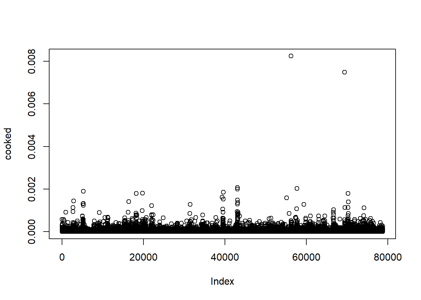

Just out of curiosity.. what were those games:

index <- names(cooked[cooked > 0.006])

nba[index,] %>%
  select(PLAYER_NAME,GAME_DATE, PTS, FG2A, FG3A, FTA, OREB)

## # A tibble: 2 x 7
##   PLAYER_NAME    GAME_DATE    PTS  FG2A  FG3A   FTA  OREB
##   <chr>          <date>     <int> <int> <int> <int> <int>
## 1 Andre Drummond 2016-01-20    17     4     0    36     5
## 2 DeAndre Jordan 2015-11-30    18     6     0    34     9

Ahh, the hack-a-center games… makes total sense. 36 and 34 free throws.

Scaling variables

Finally, we may want to scale variables to common range, using standardization ( for example to 0:1 or -1:1 range) or normalization (Z-score) to obtain variables from the same range of values. That ensures model will not be skewed by one variable having totally different scale from the rest.

Correlation based feature selection

## preparing data
ds <- nba %>%
  select(PTS,FG2A, FG3A, FTA, AST, OREB, PF, TOV, STL, PACE) %>% as.data.frame()

## correlation matrix
cm <- cor(ds)
corrplot::corrplot(cm, method = 'number', diag = F, type = 'upper')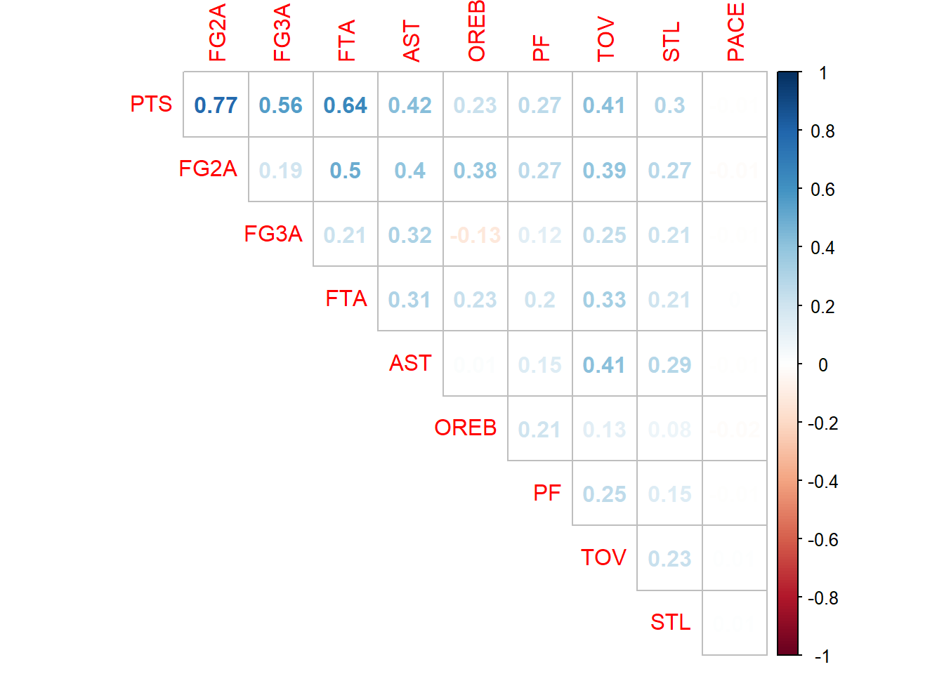 

Correlation matrix shows that variable Pace is uncorrelated with PTS at all. At least 5 variables seem to well correlated to PTS, there is no reason to be overly worried by multicollinearity. For beginning I will pick all variables except Pace and see what happens.

ds <- ds %>%
  select( - PACE)

First basic model

## defining learning task
task <- makeRegrTask(id = 'nba', data  = ds, target = 'PTS')

## defining learner: simple linear regression
learner <- makeLearner(cl = 'regr.lm')

## This time keeping things simple, going with simple holdout validation
ho <- makeResampleInstance("Holdout",task)
task_train <- subsetTask(task, ho$train.inds[[1]])
task_test <- subsetTask(task, ho$test.inds[[1]])

## Training basic model with all variables, without any transformations and tests:
model_trained_0 <- train(learner, task_train)
newdata_pred_0 <- predict(model_trained_0, task_test)

## Check RMSE, MSE and R^2
performance(newdata_pred_0,  measures = list(mse,rmse,rsq))

##       mse      rmse       rsq 
## 11.003556  3.317161  0.831295

Let’s check using cross validation

rdesc <- makeResampleDesc(method = "RepCV", reps = 2, folds = 5)
## instance for the splitting to check all models on the same conditions
rin = makeResampleInstance(rdesc, task = task)

## fourth, resample:

r <- resample(
              learner = learner,
              task = task,
              resampling = rdesc, 
              measures = list(mse,rmse,rsq),
              models = T, show.info = FALSE
              )
print(r)

## Resample Result
## Task: nba
## Learner: regr.lm
## Aggr perf: mse.test.mean=10.9240522,rmse.test.rmse=3.3051554,rsq.test.mean=0.8298947
## Runtime: 1.2772

R-squared is quite high, RMSE on training dataset looks decent… lets check the real vs predicted plot:

plotResiduals(newdata_pred_0)

## `geom_smooth()` using method = 'gam' and formula 'y ~ s(x, bs = "cs")'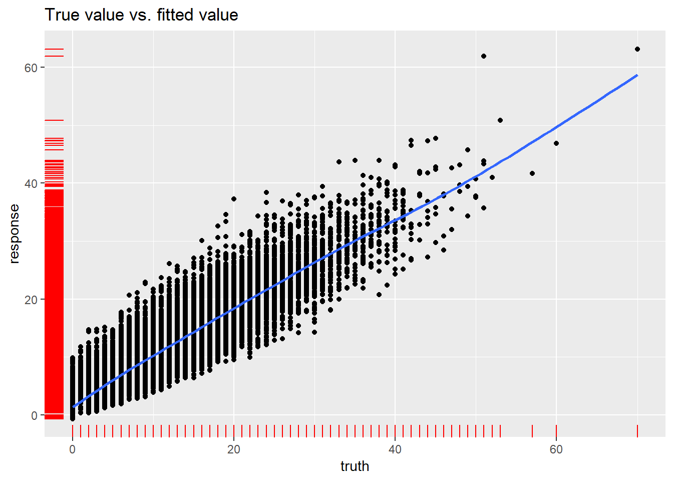

broom::tidy(model_trained_0$learner.model)

##          term    estimate   std.error  statistic
## 1 (Intercept) -0.47108412 0.029499382 -15.969287
## 2        FG2A  1.01131207 0.004328380 233.646765
## 3        FG3A  1.19560942 0.006020440 198.591693
## 4         FTA  0.80804045 0.006176252 130.830223
## 5         AST -0.04341453 0.007031087  -6.174655
## 6        OREB -0.05337875 0.012183867  -4.381101
## 7          PF  0.06146833 0.010627657   5.783808
## 8         TOV  0.04661127 0.012127939   3.843297
## 9         STL  0.02186359 0.015847430   1.379630
##                                                             p.value
## 1 0.000000000000000000000000000000000000000000000000000000002855204
## 2 0.000000000000000000000000000000000000000000000000000000000000000
## 3 0.000000000000000000000000000000000000000000000000000000000000000
## 4 0.000000000000000000000000000000000000000000000000000000000000000
## 5 0.000000000667927418573255173364633385801880649523809552192687988
## 6 0.000011830962164933312005463128535609484970336779952049255371094
## 7 0.000000007344145980840371659616877542120505495404358953237533569
## 8 0.000121535563116167445989884710044748317159246653318405151367187
## 9 0.167706448485313130980500773148378357291221618652343750000000000

First thought: there are outliers that should be treated, but first lets find out what the residuals plots present:

plot(model_trained_0$learner.model, which = 1)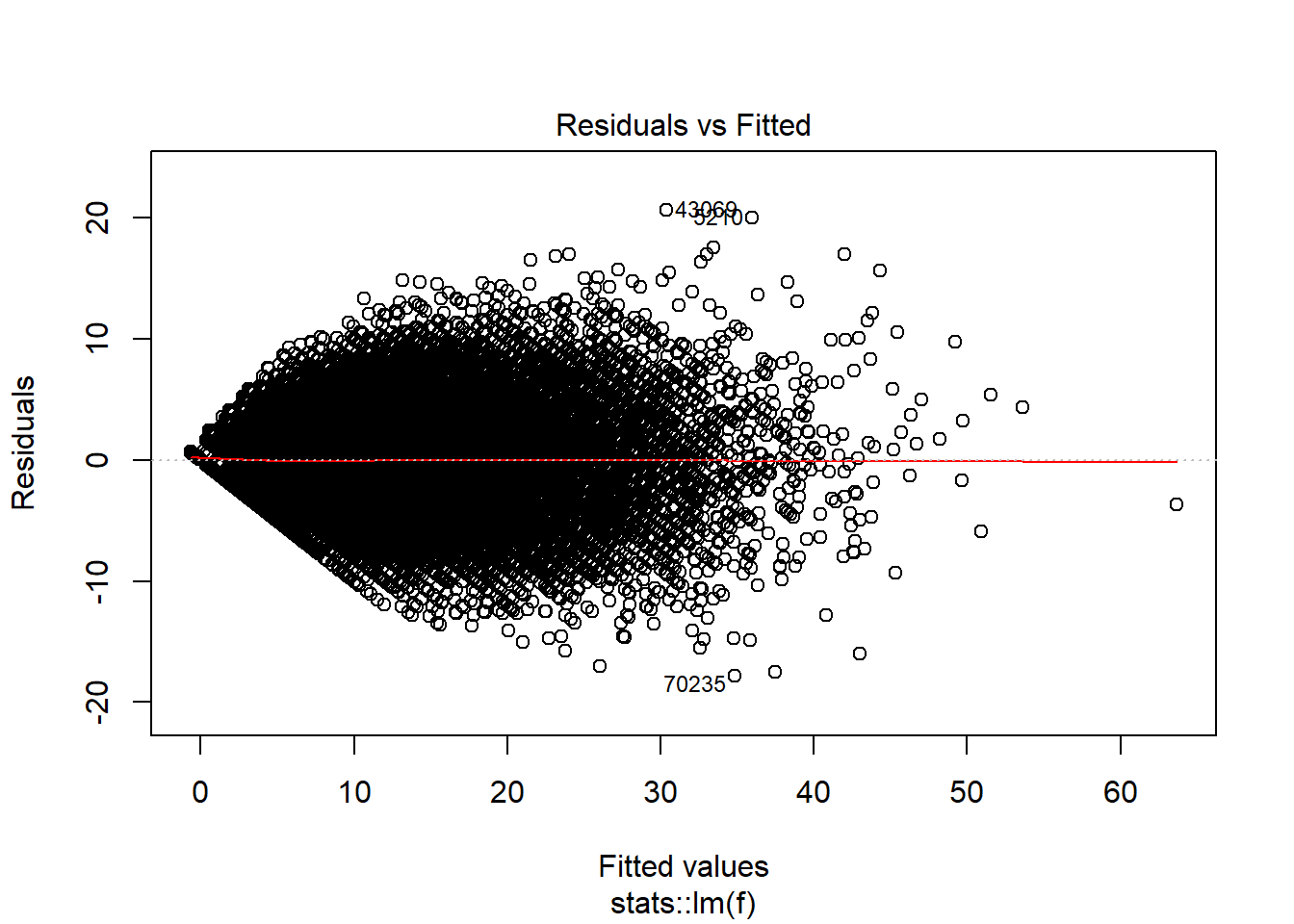

Residuals are close to show normal distribution for values between 10 and 30, but outside of that range it is not so nice.

plot(model_trained_0$learner.model, which = 2)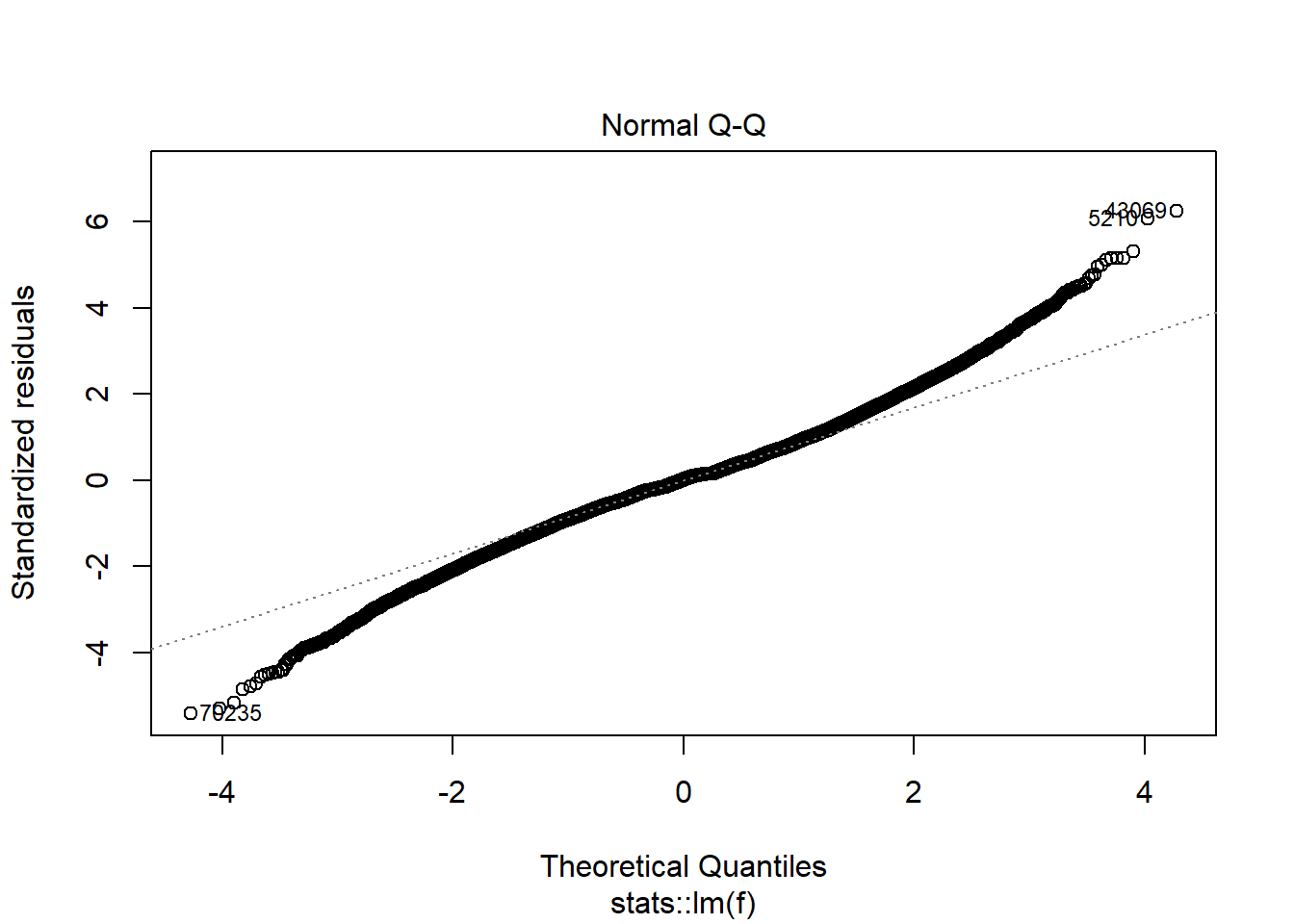

Distribution of residuals is definately not normal.

plot(model_trained_0$learner.model, which = 3)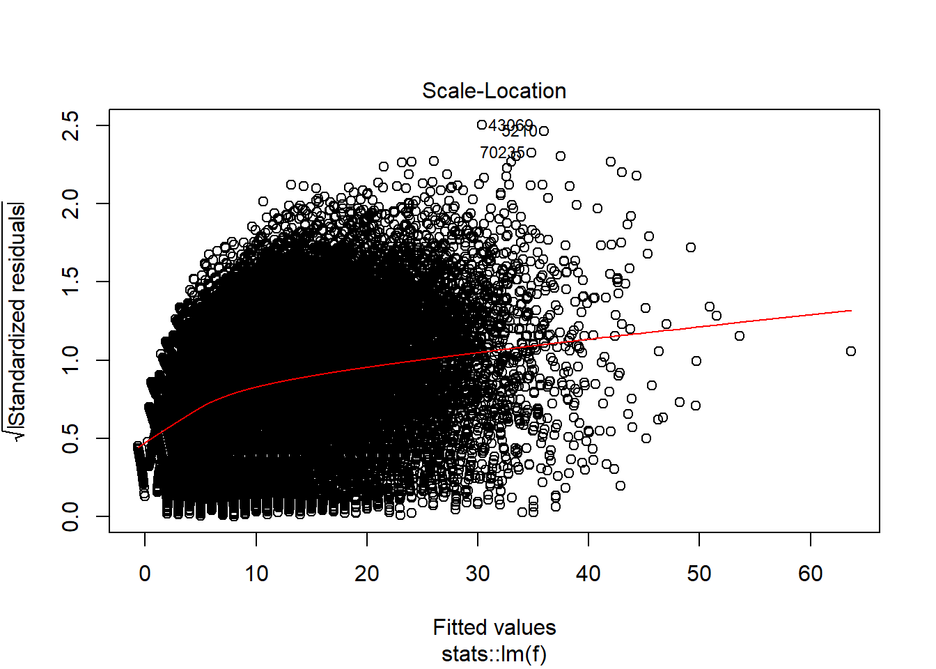

There is heteroscedaskicity as well

plot(model_trained_0$learner.model, which = 4)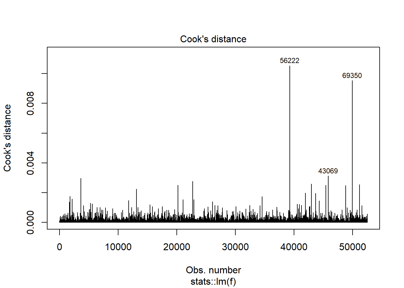

Woooh…

Let’s also run statistical test for each effect, just to have confirmation.

lmtest::bptest(model_trained_0$learner.model)

## 
##  studentized Breusch-Pagan test
## 
## data:  model_trained_0$learner.model
## BP = 7635, df = 8, p-value < 0.00000000000000022

lmtest::dwtest(model_trained_0$learner.model)

## 
##  Durbin-Watson test
## 
## data:  model_trained_0$learner.model
## DW = 2.0086, p-value = 0.8369
## alternative hypothesis: true autocorrelation is greater than 0

shapiro.test(model_trained_0$learner.model$residuals[1:5000])

## 
##  Shapiro-Wilk normality test
## 
## data:  model_trained_0$learner.model$residuals[1:5000]
## W = 0.98784, p-value < 0.00000000000000022

So:

Heterescedaskicity: check Non-normal distribution: check Outliers/Influential observations: check Autocorrelation: no..yay!

I am going to start with removing influential observations and outliers - there is a chance it will reduce other negative effects.

Model with excluded/scaled observations

I want to do 4 steps:

• Remove influential observations measured by cook’s distance
• Remove outliers in Points and Free throws
• Use only FTA, FG2A and FG3A as they have decent correlation with PTS
• Log scale predictors, since they distributions are skewed to the right

index2 <- as.numeric(names(cooked[cooked > 0.001])) ## removing by cook distance
index3 <- which(ds$PTS > 50)                   ## removing outliers
index4 <- which(ds$FTA > 15) ## removing outliers

ds_tmp0 <- ds[ - c(index2, index3, index4),c('PTS','FTA','FG2A','FG3A')]

ds_tmp0 <- ds_tmp0 %>% 
  mutate(FG3A = log(FG3A),
         FTA = log(FTA),
         FG2A = log(FG2A)
         )
         
is.na(ds_tmp0) <- sapply(ds_tmp0, is.infinite)
ds_new <- ds_tmp0 %>% tidyimpute::impute_zero()


task <- makeRegrTask(id = 'nba', data  = ds_new, target = 'PTS')

learner <- makeLearner(cl = 'regr.lm')

## This time keeping things simple, going with simple holdout validation
ho <- makeResampleInstance("Holdout",task)
task_train <- subsetTask(task, ho$train.inds[[1]])
task_test <- subsetTask(task, ho$test.inds[[1]])

## Training basic model with all variables, without any transformations and tests:
model_trained_0 <- train(learner, task_train)
newdata_pred_0 <- predict(model_trained_0, task_test)

## Check RMSE, MSE and R^2
performance(newdata_pred_0,  measures = list(mse,rmse,rsq))

##       mse      rmse       rsq 
## 15.675226  3.959195  0.748217

plotResiduals(newdata_pred_0)

## `geom_smooth()` using method = 'gam' and formula 'y ~ s(x, bs = "cs")'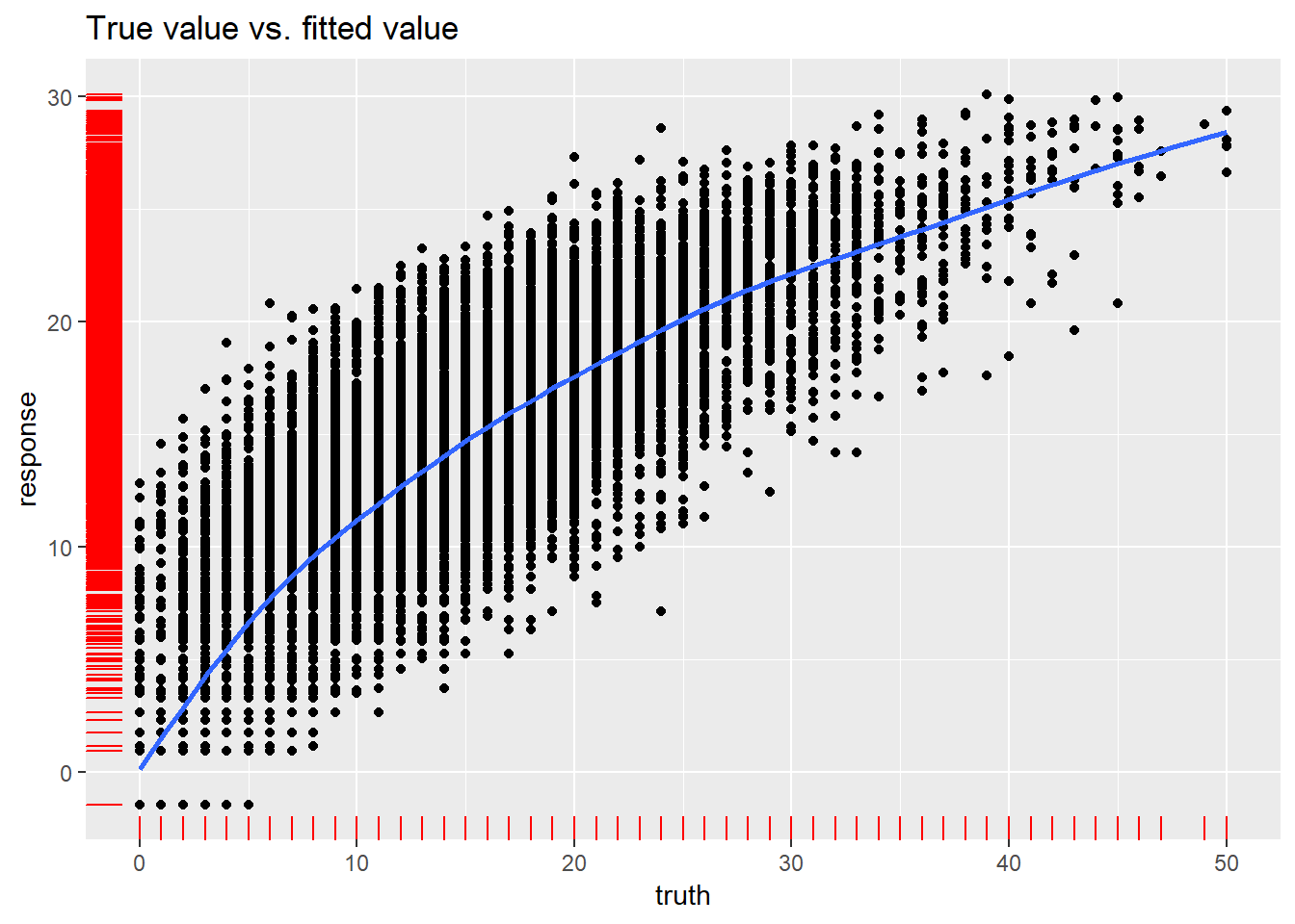

Let’s check using cross validation again

rdesc <- makeResampleDesc(method = "RepCV", reps = 2, folds = 5)
## instance for the splitting to check all models on the same conditions
rin = makeResampleInstance(rdesc, task = task)

## fourth, resample:

r <- resample(
              learner = learner,
              task = task,
              resampling = rdesc, 
              measures = list(mse,rmse,rsq),
              models = T, show.info = FALSE
              )
print(r)

## Resample Result
## Task: nba
## Learner: regr.lm
## Aggr perf: mse.test.mean=15.3804608,rmse.test.rmse=3.9217931,rsq.test.mean=0.7531529
## Runtime: 0.542082

plot(model_trained_0$learner.model, which = 1)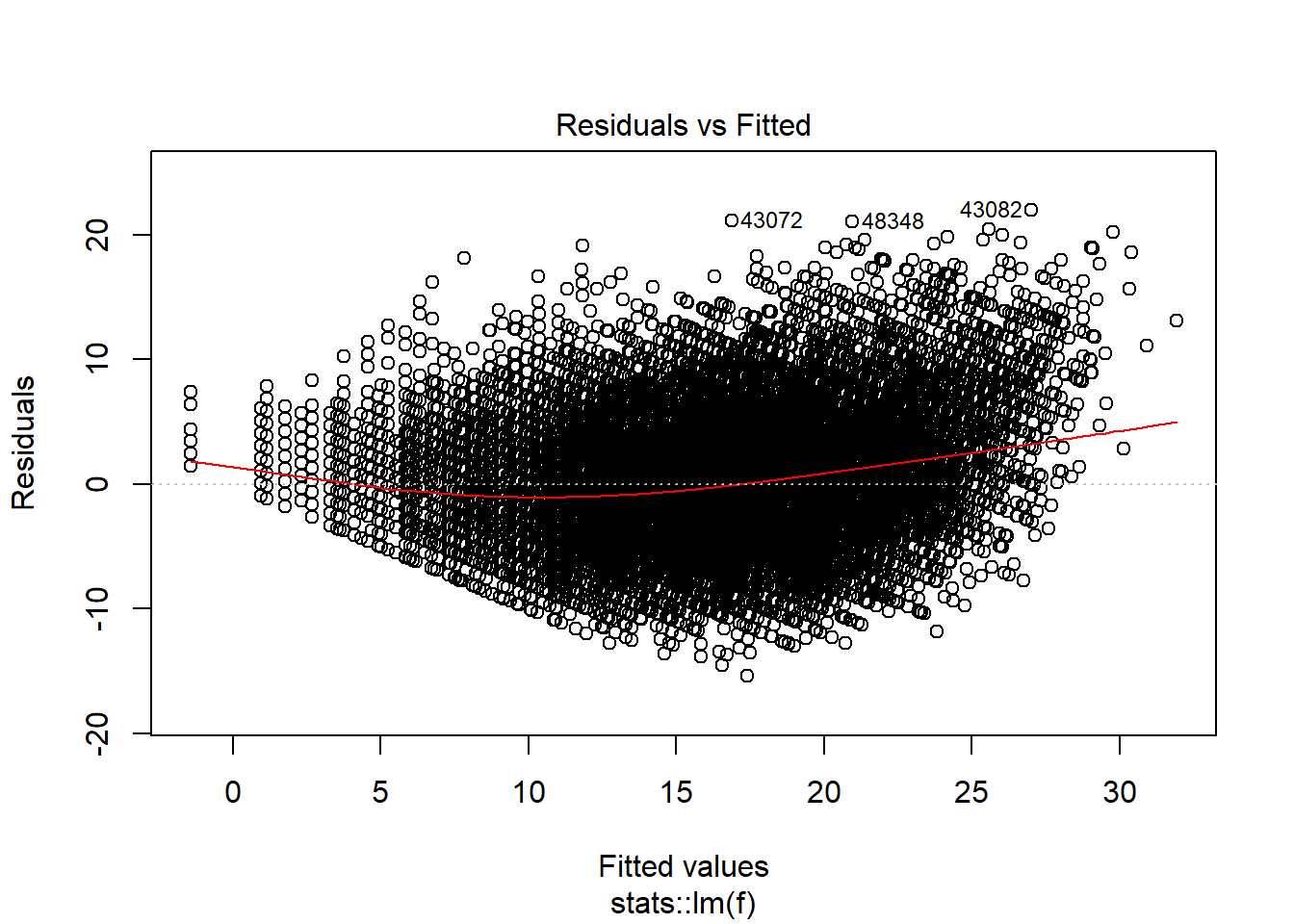

plot(model_trained_0$learner.model, which = 2)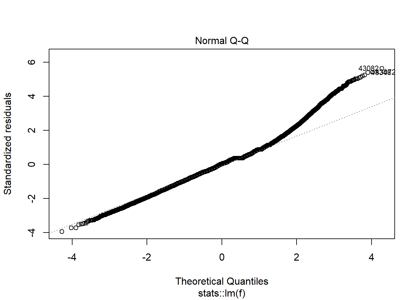

plot(model_trained_0$learner.model, which = 3)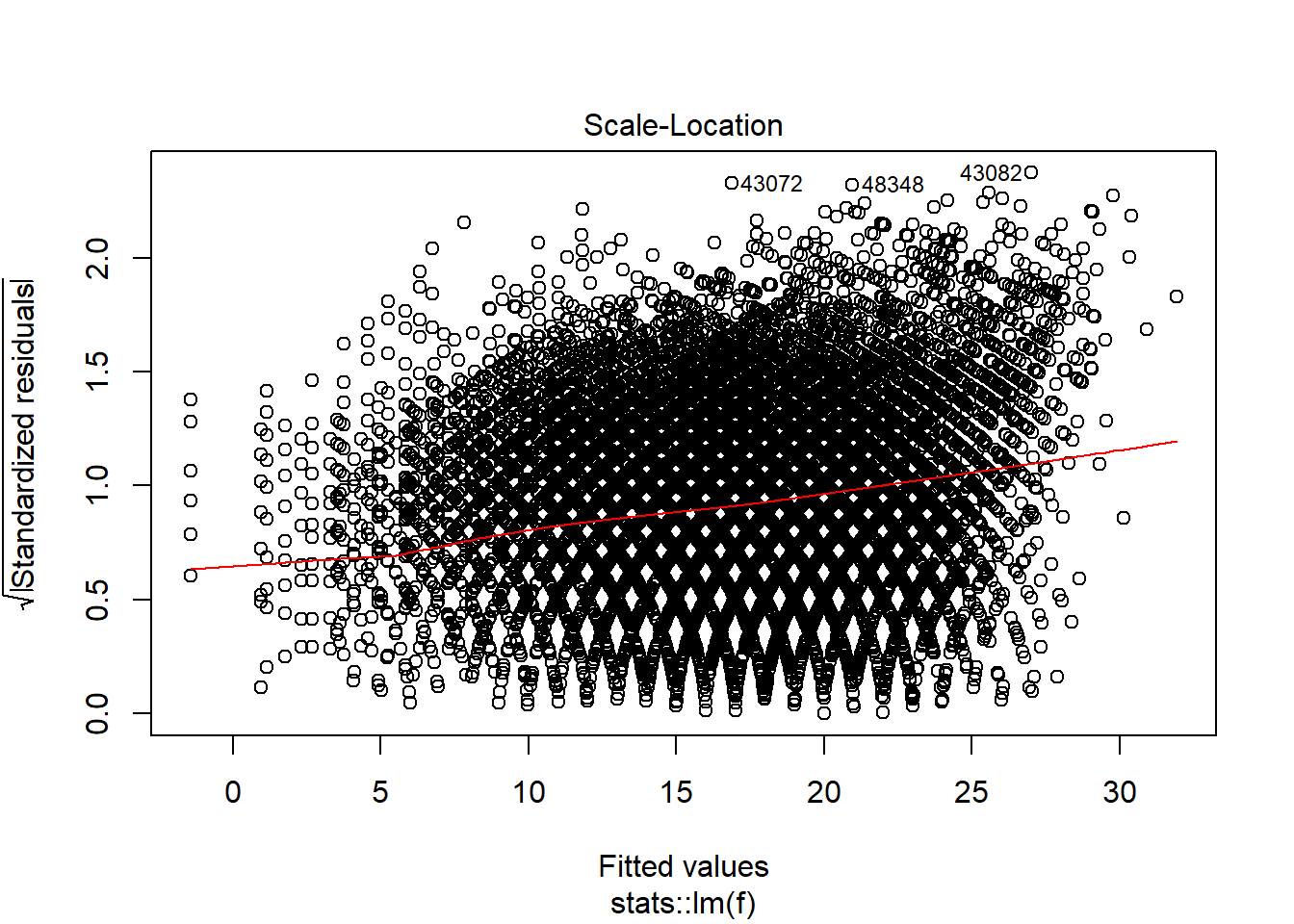

Transformations helped lower heteroscedaskicity and non normal distribution for observations which has value of Points no larger than 30-35. There is still problem affecting high-scoring performances.

Even though model performance metrics are worse for the second model, I think that tweaked version has better quality of prediction, especially for lower values of points. What would help solve the issue, is another variable describing if given player is an all-star (those players are more likely to score over 30 points).

Another possibility is to use split the model into 2: one working for lower PTS values, one for larger.